Introduction to geometric systems theory

 Linear geometric systems (control) theory was initiated in the beginning of the 1970's (see Basile and Marro). A good summary of the subject is the book by Wonham.

The term ``geometric'' suggests several things. First it suggests that the setting is linear state space and the mathematics behind is primarily linear algebra (with a geometric flavor). Secondly it suggests that the underlying methodology is geometric. It treats many important system concepts, for example controllability, as geometric properties of the state space or its subspaces. These are the properties that are preserved under coordinate changes, for example, the so-called invariant or controlled invariant subspaces. On the other hand, we know that things like distance and shape do depend on the coordinate system one chooses. Using these concepts the geometric approach captures the essence of many analysis and synthesis problems and treat them in a coordinate-free fashion. By characterizing the solvability of a control problem as a verifiable property of some constructible subspace, calculation of the control law becomes much easier. In many cases, the geometric approach can convert what is usually a difficult nonlinear problem into a straight-forward linear one.

The linear geometric systems theory was extended to nonlinear systems in the 1970's and 1980's (see the book by Isidori). The underlying fundamental concepts are almost the same, but the mathematics is different. For nonlinear systems the tools from differential geometry are primarily used.

In the rest of the chapter, we use some typical problems and examples to illustrate the advantages and basic ideas of geometric approaches.

Let us start with an example of a linear system. The purpose of the example is to show that we can model even quite complex practical systems as linear systems.

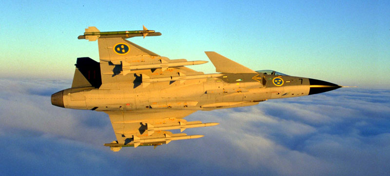
Example: Longitudinal motions of an aircraft

By longitudinal motions of an aircraft we mean, the movement of an aircraft as if it were constrained to move exclusively in a vertical plane. This is a very important type of motion of an aircraft. It is possible to show that under perfect geometrical and dynamical symmetry conditions, the linearized equations of motion of any aircraft exhibit an exact longitudinal-lateral decoupling. The full explanation of the model equations falls outside the scope of this work, and can be found in (Etkin).

In our notations, V stands for the velocity modulus, m is the mass of the aircraft, T is the thrust force exerted by the engines and supposed to be acting along the main body axis, D is the magnitude of the total aerodynamic drag acting opposite to the velocity vector, L is the total aerodynamic magnitude of the lift force in an orthogonal direction to the velocity, mg is the gravity force acting at the center of gravity (CG) and pointing downwards (flat Earth approximation). M_y is the total pitching moment around the axis perpendicular to the plane of movement, $\alpha$ is the angle of attack of the aircraft (angle between the velocity and the x-axis), $\gamma$ is the angle of climb (between the horizontal axis and the velocity), and $\theta = \gamma + \alpha$ is the pitch angle of the aircraft. By convention, the pitch rate ($\dot \theta$ in the longitudinal motions) is denoted q.

  

Figure 1.1: Variables for the aircraft model.

The linearized equations of motion are:
 

$$\begin{array} {lcl} m \Delta \dot V & = & \Delta T - mg \cos... ...iptsize ATP} }}\Delta T\\ \Delta \dot \theta & = & q\end{array}$$ (1)

These are differential equations in incremental variables with respect to any admissible equilibrium condition (denoted with subscripts e). For example, $V = V_e + \Delta V; \quad \gamma = \gamma_e + \Delta \gamma; \quad \alpha = \alpha_e + \Delta \alpha$. Around each flight equilibrium condition, the pilot can control whether to increase or decrease the thrust of the engines which is $\Delta T$. This he (or she) does by adjusting the throttle lever. If he wants to correct the attitude of the aircraft, he deflects the stick, leading to changes in the deflection angles of the elevator and Canards if the airplane has Canards. An equivalent version of (1.1) written in compact vector notation is
 

$${\bf \Delta \dot x} = {\bf A}{\bf \Delta x} + {\bf B}{\bf \Delta u}$$ (2)

The elevator and Canard actuator dynamics are assumed so fast, that no states are used to represent them. The situation is depicted in Fig. 1.2. Thus, neglected actuator dynamics means here $u_1 = \mbox{$\delta_{E}$}$ and $u_2 = \mbox{$\delta_{C}$}$. Notice that in this model, the first two states are not $\Delta V$ and $\Delta \gamma$ as in (1.1).

  

Figure 1.2: Detailed system architecture

Naturally, we need to include external disturbances such as turbulence to make the model complete.

Here are a few samples of the problems we will study in this course.

Problem: Disturbance decoupling

Consider the system
 

$$\begin{array} {rcl} \dot x&=&Ax+Bu+Ew \\ y&=&Cx,\end{array}$$ (3)

where u is the control signal and w is an external disturbance that cannot be measured. The question is if there exits a state feedback

u=Fx+v

such that the output y is unaffected by the disturbance w.

Suppose such a feedback exists. Then by plugging in the control, we have

$$\begin{array} {rcl} \dot x&=&(A+BF)x+Bv+Ew \\ y&=&Cx.\end{array}$$ (4)

The fact that the output y is unaffected by the disturbance w implies that the nth derivative y⁽ⁿ⁾(t) for any $n \ge 1$ and any t does not depend on w. Since

y⁽ⁿ⁾(t)=C(A+BF)ⁿx(t)+C(A+BF)^n-1Bv(t)+C(A+BF)^n-1Ew(t),

(here we assume v and w are constants for the sake of simplicity) we must have

$$C(A+BF)^{n-1}E=0,~~\forall n\ge 1.$$

In other words, if we can find an F that satisfies the above equations, then the problem is solved.

However, the equations are highly nonlinear, thus difficult to solve. In Chapter 3 we will use the idea of ``controlled invariance'' to reduce the problem into a linear one.

Problem: Output regulation

Consider

$$\begin{array} {rcl} \dot x&=&Ax+Bu+Ew \\ e&=&Cx-Dw,\end{array}$$ (5)

where w models both the disturbance to reject and the reference signal to track (We can consider y=Cx as the output. Thus w₁=Dw is the reference to track, while the rest of w is disturbance). Furthermore, we assume that w is generated by the following system:

$$\dot w=\Gamma w.$$ (6)

A system that generates an input signal is sometimes called an exogenous system . The problem of output regulation is to find a feedback control law such that the closed-loop system is asymptotically stable when w is set to zero and such that e(t) tends to zero as t tends to $\infty$.

The difference with the disturbance decoupling problem is that here we only require the output to reject the disturbance in the steady state, and we also have some knowledge about the disturbance. The discussion of this problem in Chapter 7 will lead to the famous ``internal model principle'' (Wonham and Francis). Surprisingly we will show that this problem is generically solvable while the disturbance decoupling problem is not. Not surprisingly, the idea of controlled invariance also plays a central role here.

Problem: Controllability under constraints

Consider the system
 

$$\begin{array} {rcl} \dot x&=&Ax+Bu \\ y&=&Cx,\end{array}$$ (7)

Let $\mathcal{K}$ be a subspace of $\mathbb R^n$. The question is which subset $\mathcal{R}\subseteq \mathcal{K}$ can be reached in finite time t₁ from any initial point in $\mathcal{K}$ with controls of the form

u=Fx+Gv,

if we require that the trajectory $\{x(t): t \in [0,t_1]\}$ should be in $\mathcal{K}$.

This problem is quite relevant in many applications, for example, in path planning for mobile systems.

In this set of lecture notes, we will also discuss some system concepts for nonlinear systems. We give an example here to illustrate why sometimes one has to use nonlinear tools.

Example: Car steering

The steering system of a car can be modeled as

  

Figure 1.3: The geometry of the car-like robot, with position (x,y), orientation $\theta$ and steering angle $\phi$.

 

$$\begin{array} {rcl} \dot{x} &=& v \cos (\theta) \\ \dot... ...heta) \\ \dot{\theta} &=& \frac{v}{l} \tan \phi,\\ \end{array}$$ (8)

where x and y are cartesian coordinates of the middle point on the rear axle, $\theta$ is the orientation angle, v is the longitudinal velocity measured at that point, l is the distance of the two axles, and $\phi$ is the steering angle. In this case v and $\phi$ are the two controls.

Let us reduce the complexity by defining u₁=v, $u_2=\frac{v}{l} \tan \phi$, then
 

$$\begin{array} {rcl} \dot{x} &=& \cos (\theta)u_1 \\ \dot{y} &=& \sin (\theta)u_1 \\ \dot{\theta} &=& u_2.\\ \end{array}$$ (9)

Sometimes, this is called a unicycle model. If we linearize (1.9) around a point $(x_0,y_0,\theta_0)$, we have
 

$$\begin{array} {rcl} \dot{x} &=& \cos (\theta_0)u_1 \\ \d... ... &=& \sin (\theta_0)u_1 \\ \dot{\theta} &=& u_2,\\ \end{array}$$ (10)

which is not controllable. However, using geometric tools we will show in Chapter 8 that the nonlinear system (1.9) is controllable (This is what you, as a driver, expected, right?).

The notes are organized as follows.

In Chapter 2, invariant and controlled invariant subspaces will be discussed; In Chapter 3, the disturbance decoupling problem will be introduced; In Chapter 4, we will introduce transmission zeros and their geometric interpretations; In Chapter 5, noninteracting control and tracking will be studied as applications of the zero dynamics normal form; In Chapter 6, we will discuss some input-output behaviors from a geometric point of view; In Chapter 7, we will discuss the output regulator problem in some detail. Finally, in Chapter 8, we will extend some of the central concepts in the geometric control to nonlinear systems.